交互式旋转链排列相互作用驱动场 AHS 程序在本地模拟器上运行分析模拟器结果 Run QuEra ning on 的 Aquila QPU 分析结果后续步骤

Hello AHS：运行您的第一个模拟哈密顿模拟

本节提供了有关运行第一个模拟哈密顿模拟的信息。

本节内容：

交互式旋转链
排列
相互作用
驱动场
AHS 程序
在本地模拟器上运行
分析模拟器结果
Run QuEra ning on 的 Aquila QPU
分析结果
后续步骤

交互式旋转链

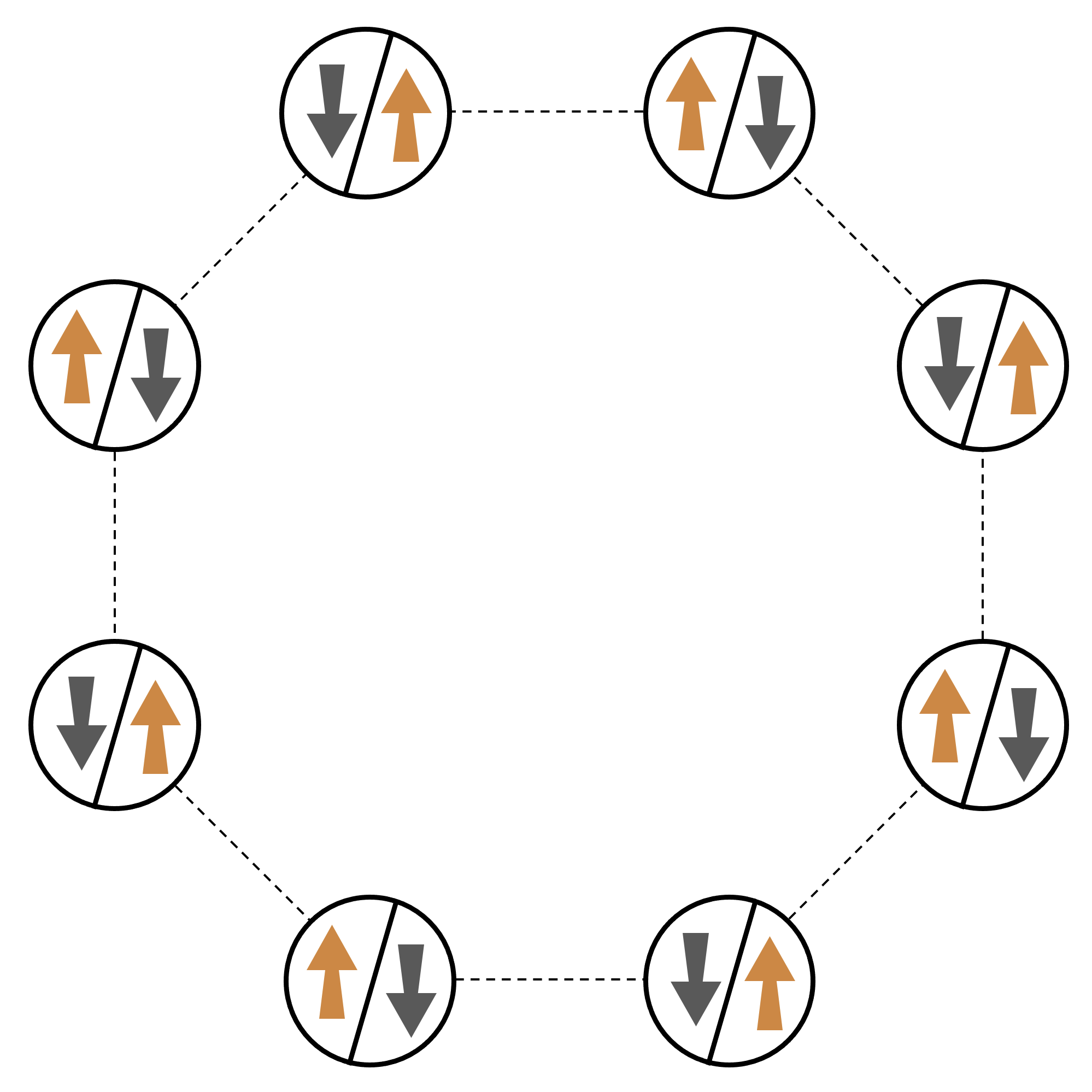
举一个由许多相互作用粒子组成的系统的典型示例，让我们考虑一个由八个旋转组成的环（每个旋转都可以处于“向上”∣↑⟩ 和“向下”∣↓⟩ 的状态）。尽管规模很小，但该模型系统已经表现出自然存在的磁性材料的一些有趣现象。在此例中，我们将展示如何准备一个所谓的反铁磁阶数，即连续的自旋指向相反的方向。

排列

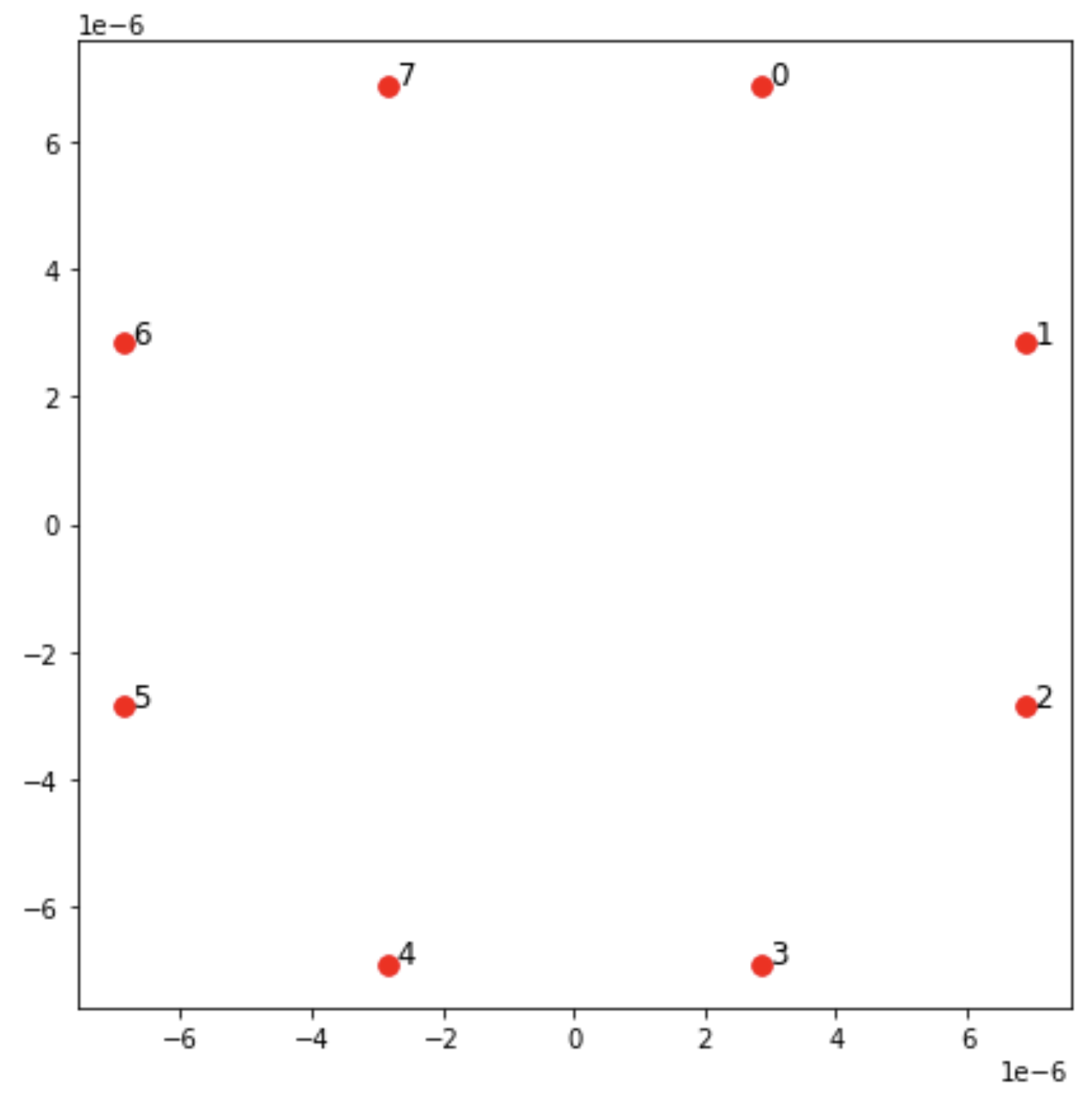
我们将使用一个中性原子来代表每次自旋，“向上”和“向下”自旋态将分别以激发的里德伯格态和原子的基态编码。首先，创建二维排列。我们可以用以下代码对上面的旋转圈进行编程。

先决条件：您需要 pip 安装 Braket SDK。（如果您使用的是 Braket 托管的笔记本实例，则此 SDK 已预先安装在笔记本中。）要重现绘图，您还需要使用 shell 命令 pip install matplotlib 单独安装 matplotlib。


from braket.ahs.atom_arrangement import AtomArrangement
import numpy as np
import matplotlib.pyplot as plt  # Required for plotting

a = 5.7e-6  # Nearest-neighbor separation (in meters)

register = AtomArrangement()
register.add(np.array([0.5, 0.5 + 1/np.sqrt(2)]) * a)
register.add(np.array([0.5 + 1/np.sqrt(2), 0.5]) * a)
register.add(np.array([0.5 + 1/np.sqrt(2), - 0.5]) * a)
register.add(np.array([0.5, - 0.5 - 1/np.sqrt(2)]) * a)
register.add(np.array([-0.5, - 0.5 - 1/np.sqrt(2)]) * a)
register.add(np.array([-0.5 - 1/np.sqrt(2), - 0.5]) * a)
register.add(np.array([-0.5 - 1/np.sqrt(2), 0.5]) * a)
register.add(np.array([-0.5, 0.5 + 1/np.sqrt(2)]) * a)

我们还可以绘制散点图，


fig, ax = plt.subplots(1, 1, figsize=(7, 7))
xs, ys = [register.coordinate_list(dim) for dim in (0, 1)]
ax.plot(xs, ys, 'r.', ms=15)

for idx, (x, y) in enumerate(zip(xs, ys)):
    ax.text(x, y, f" {idx}", fontsize=12)

plt.show()  # This will show the plot below in an ipython or jupyter session

相互作用

为准备反铁磁相，我们需要诱导相邻自旋之间的相互作用。为此，我们使用了 van der Waals 相互作用，该相互作用是由中性原子设备（如来自 QuEra 的 Aquila 设备）原生实现的。这种相互作用的哈密顿项使用自旋表示，可以表示为所有自旋对 (j,k) 的总和。

其中：nj=∣↑_j⟩⟨↑_j∣ 是一个运算符，仅当自旋 j 处于“向上”状态时才取值 1，否则取值 0。强度为 V_j,k=C₆/(d_j,k)⁶，其中：C₆ 是固定系数，d_j,k 是自旋 j 和 k 之间的欧几里得距离。这个相互作用项的直接影响是，任何自旋 j 和自旋 k 都是“向上”状态的能量都会升高（按量 V_j,k）。通过精心设计 AHS 程序的其余部分，这种相互作用可防止相邻的旋转都处于“向上”状态，这种效果通常被称为“Rydberg 阻塞”。

驱动场

AHS 程序开始时，所有旋转（默认情况下）都以“向下”状态开始，它们处于所谓的铁磁阶段。着眼于准备反铁磁相位的目标，我们指定了一个时变相干驱动场，该驱动场可以平稳地将自旋从这种状态过渡到多体状态，首选为“向上”状态。相应的哈密顿量可以写成

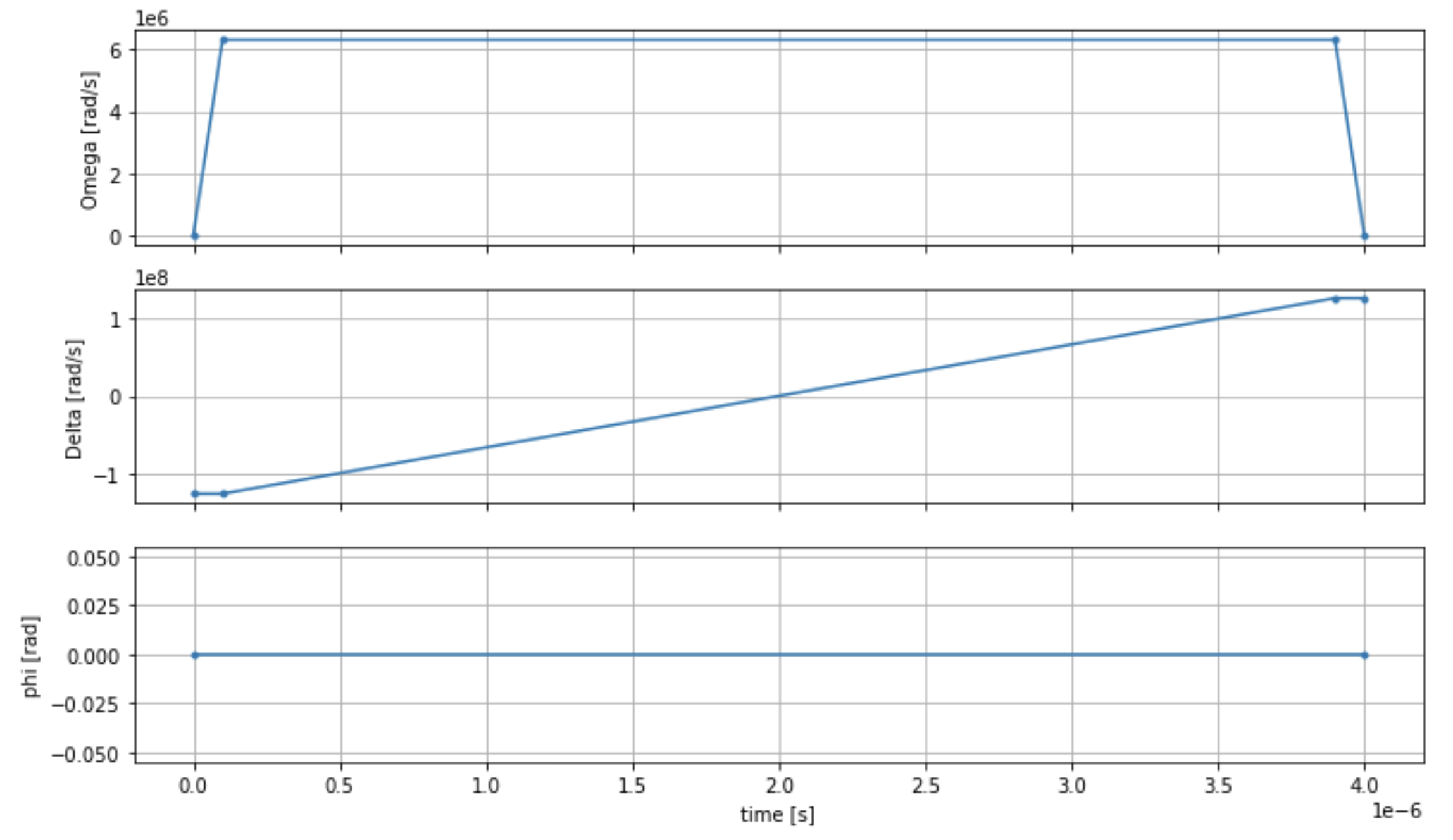
其中 Ω(t)、(t)、Δ(t) 是时变全局振幅（又名 Rabi 频率）、相位和失谐均匀地影响所有自旋的驱动场。其中：S_−,k =∣↓_k⟩⟨↑_k∣and S_+,k=(S_−,k)^†=∣↑_k⟩⟨↓_k∣分别是 spin k 的降低和升高运算符，n_k=∣↑_k⟩⟨↑_k∣和以前的运算符相同。驱动场的 Ω 部分同时连贯地耦合所有旋转的“向下”和“向上”状态，而 Δ 部分控制“向上”状态的能量奖励。

为了对从铁磁相向到反铁磁相的平滑过渡进行编程，我们使用以下代码指定驱动场。


from braket.timings.time_series import TimeSeries
from braket.ahs.driving_field import DrivingField

# Smooth transition from "down" to "up" state
time_max = 4e-6  # seconds
time_ramp = 1e-7  # seconds
omega_max = 6300000.0  # rad / sec
delta_start = -5 * omega_max
delta_end = 5 * omega_max

omega = TimeSeries()
omega.put(0.0, 0.0)
omega.put(time_ramp, omega_max)
omega.put(time_max - time_ramp, omega_max)
omega.put(time_max, 0.0)

delta = TimeSeries()
delta.put(0.0, delta_start)
delta.put(time_ramp, delta_start)
delta.put(time_max - time_ramp, delta_end)
delta.put(time_max, delta_end)

phi = TimeSeries().put(0.0, 0.0).put(time_max, 0.0)

drive = DrivingField(
   amplitude=omega,
   phase=phi,
   detuning=delta
)

我们可以使用以下脚本可视化驱动场的时间序列。


fig, axes = plt.subplots(3, 1, figsize=(12, 7), sharex=True)

ax = axes[0]
time_series = drive.amplitude.time_series
ax.plot(time_series.times(), time_series.values(), '.-')
ax.grid()
ax.set_ylabel('Omega [rad/s]')

ax = axes[1]
time_series = drive.detuning.time_series
ax.plot(time_series.times(), time_series.values(), '.-')
ax.grid()
ax.set_ylabel('Delta [rad/s]')

ax = axes[2]
time_series = drive.phase.time_series
# Note: time series of phase is understood as a piecewise constant function
ax.step(time_series.times(), time_series.values(), '.-', where='post')
ax.set_ylabel('phi [rad]')
ax.grid()
ax.set_xlabel('time [s]')

plt.show()  # This will show the plot below in an ipython or jupyter session

三张图显示了一段时间内的 phi、delta 和 omega。顶部的子图显示增长到略高于 6， rads/s 在此处它保持 4 秒钟，直到回落到 0。中间的图描绘了导数的相关线性增长，底图描绘了一条接近零的平线。

AHS 程序

寄存器、驱动场（以及隐式的范德华相互作用）构成了模拟哈密顿模拟程序 ahs_program。


from braket.ahs.analog_hamiltonian_simulation import AnalogHamiltonianSimulation

ahs_program = AnalogHamiltonianSimulation(
   register=register,
   hamiltonian=drive
)

在本地模拟器上运行

由于此示例很小（少于 15 次旋转），因此在兼容 AHS 的 QPU 上运行之前，我们可以在 Braket SDK 附带的本地 AHS 模拟器上运行它。由于本地模拟器可免费使用 Braket SDK，因而这是确保我们的代码能够正确执行的最佳实践。

在这里，我们可以将拍摄次数设置为较大的值（比如 100 万），因为本地模拟器会跟踪量子态的时间演变并从最终状态中抽取样本；因此，可以增加拍摄次数，而总运行时仅略有增加。


from braket.devices import LocalSimulator

device = LocalSimulator("braket_ahs")

result_simulator = device.run(
   ahs_program,
   shots=1_000_000
).result()  # Takes about 5 seconds

分析模拟器结果

我们可以使用以下函数汇总拍摄结果，该函数可以推断每次旋转的状态（可以是“d”代表“向下”，“u”表示“向上”，“e“代表空场地），并计算每种配置在拍摄中发生的次数。


from collections import Counter


def get_counts(result):
    """Aggregate state counts from AHS shot results

    A count of strings (of length = # of spins) are returned, where
    each character denotes the state of a spin (site):
      e: empty site
      u: up state spin
      d: down state spin

    Args:
      result (braket.tasks.analog_hamiltonian_simulation_quantum_task_result.AnalogHamiltonianSimulationQuantumTaskResult)

    Returns
       dict: number of times each state configuration is measured

    """
    state_counts = Counter()
    states = ['e', 'u', 'd']
    for shot in result.measurements:
        pre = shot.pre_sequence
        post = shot.post_sequence
        state_idx = np.array(pre) * (1 + np.array(post))
        state = "".join(map(lambda s_idx: states[s_idx], state_idx))
        state_counts.update((state,))
    return dict(state_counts)


counts_simulator = get_counts(result_simulator)  # Takes about 5 seconds
print(counts_simulator)


*[Output]*
{'dddddddd': 5, 'dddddddu': 12, 'ddddddud': 15, ...}

在这里，counts 是一本字典，它计算了拍摄中观察到的每种状态配置的次数。我们还可以使用以下代码实现它们的可视化。


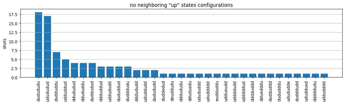
from collections import Counter


def has_neighboring_up_states(state):
    if 'uu' in state:
        return True
    if state[0] == 'u' and state[-1] == 'u':
        return True
    return False


def number_of_up_states(state):
    return Counter(state)['u']


def plot_counts(counts):
    non_blockaded = []
    blockaded = []
    for state, count in counts.items():
        if not has_neighboring_up_states(state):
            collection = non_blockaded
        else:
            collection = blockaded
        collection.append((state, count, number_of_up_states(state)))

    blockaded.sort(key=lambda _: _[1], reverse=True)
    non_blockaded.sort(key=lambda _: _[1], reverse=True)

    for configurations, name in zip((non_blockaded,
                                     blockaded),
                                    ('no neighboring "up" states',
                                     'some neighboring "up" states')):
        plt.figure(figsize=(14, 3))
        plt.bar(range(len(configurations)), [item[1] for item in configurations])
        plt.xticks(range(len(configurations)))
        plt.gca().set_xticklabels([item[0] for item in configurations], rotation=90)
        plt.ylabel('shots')
        plt.grid(axis='y')
        plt.title(f'{name} configurations')
        plt.show()


plot_counts(counts_simulator)

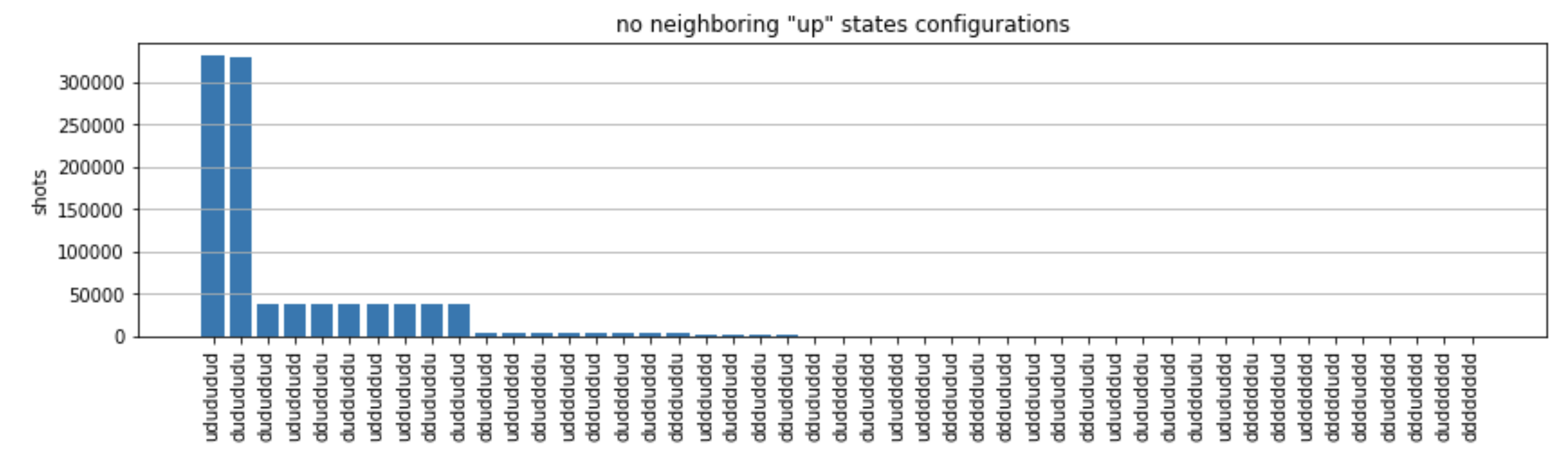
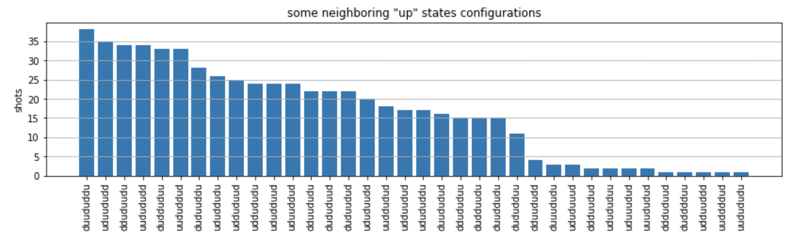
条形图显示了一些相邻的“向上”状态配置的拍摄，其中 1.0 次拍摄有 4 个状态。

从图中，我们可以读出以下观测结果，以验证我们成功制备了反铁磁相。

通常，非阻塞状态（没有两个相邻的旋转处于“向上”状态）比至少有一对相邻旋转都处于“向上”状态的状态更为常见。
通常，除非配置被阻止，否则会优先选择激励更多“向上”状态。
最常见的状态确实是完美的反铁磁态 "dudududu" 和 "udududud"。
第二种常见的状态是只有 3 个“向上”激励，连续间隔为 1、2、2 的状态。这表明范德华的相互作用也会对最近的邻居产生影响（尽管该影响要小得多）。

Run QuEra ning on 的 Aquila QPU

先决条件：除了 pip 安装 Braket SDK 之外，如果您不熟悉 Amazon Braket，请确保您已完成必要的入门步骤。

注意

如果您使用的是 Braket 托管的笔记本实例，则该实例预装了 Braket SDK。

安装所有依赖项后，我们就可以连接到 Aquila QPU 了。


from braket.aws import AwsDevice

aquila_qpu = AwsDevice("arn:aws:braket:us-east-1::device/qpu/quera/Aquila")

为了使我们的 AHS 程序适合 QuEra 机器，我们需要对所有值进行四舍五入，以符合 Aquila QPU 规定的精度水平。（这些要求受名称中带有“分辨率”的设备参数的约束。我们可以通过在笔记本中执行 aquila_qpu.properties.dict() 来看到它们。有关 Aquila 功能和要求的更多详细信息，请参阅 Aquila 笔记本简介。）我们可以通过调用 discretize 方法来做到这一点。


discretized_ahs_program = ahs_program.discretize(aquila_qpu)

现在，我们可以在 Aquila QPU 上运行该程序（目前只运行 100 次拍摄）。

注意

在 Aquila 处理器上运行此程序将产生一定的成本。Amazon Braket SDK 包含一个成本追踪器，这样，客户能够设置成本限额并近乎实时地跟踪成本。


task = aquila_qpu.run(discretized_ahs_program, shots=100)

metadata = task.metadata()
task_arn = metadata['quantumTaskArn']
task_status = metadata['status']

print(f"ARN: {task_arn}")
print(f"status: {task_status}")


*[Output]*
ARN: arn:aws:braket:us-east-1:123456789012:quantum-task/12345678-90ab-cdef-1234-567890abcdef
status: CREATED

由于量子任务的运行时差异很大（取决于可用窗口和 QPU 利用率），因此记下量子任务 ARN 是个好主意，这样我们就可以在后续时间使用以下代码片段检查其状态了。


# Optionally, in a new python session
from braket.aws import AwsQuantumTask

SAVED_TASK_ARN = "arn:aws:braket:us-east-1:123456789012:quantum-task/12345678-90ab-cdef-1234-567890abcdef"

task = AwsQuantumTask(arn=SAVED_TASK_ARN)
metadata = task.metadata()
task_arn = metadata['quantumTaskArn']
task_status = metadata['status']

print(f"ARN: {task_arn}")
print(f"status: {task_status}")


*[Output]*
ARN: arn:aws:braket:us-east-1:123456789012:quantum-task/12345678-90ab-cdef-1234-567890abcdef
status: COMPLETED

状态为“已完成”（也可以从 Amazon Braket 控制台的量子任务页面进行检查）后，我们可以通过以下方式查询结果：


result_aquila = task.result()

分析结果

我们可以使用与以前相同的 get_counts 函数计算计数。


counts_aquila = get_counts(result_aquila)
   print(counts_aquila)


*[Output]*
{'dddududd': 2, 'dudududu': 18, 'ddududud': 4, ...}

然后，用 plot_counts 绘制函数：


plot_counts(counts_aquila)

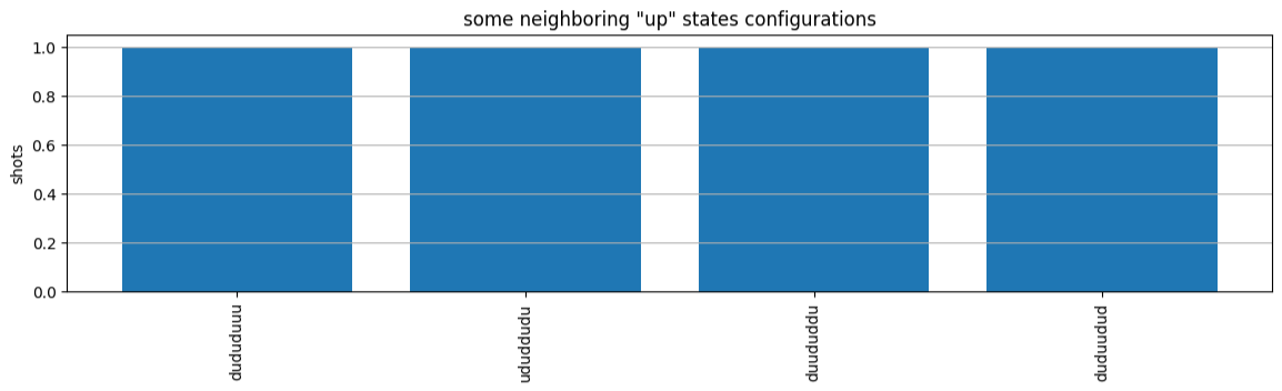
请注意，一小部分拍摄的场地为空（标为“e”）。这是由于 Aquila QPU 的每个原子制备存在 1%-2% 的缺陷。除此之外，由于拍摄次数少，结果在预期的统计波动范围内与模拟相符。

后续步骤

恭喜！您现在已经使用本地 AHS 模拟器和 Aquila QPU 在 Amazon Braket 上运行了第一个 AHS 工作负载。

要了解有关 Rydberg 物理学、模拟哈密顿模拟和 Aquila 设备的更多信息，请参阅我们的示例笔记本。

Javascript 在您的浏览器中被禁用或不可用。

要使用 Amazon Web Services 文档，必须启用 Javascript。请参阅浏览器的帮助页面以了解相关说明。

文档惯例

（高级）模拟哈密顿模拟

使用 A QuEra quila 提交模拟节目