Overview
Note
You can only view the Overview page after the forecast is generated for the first time.
The Overview tab provides the following information.
-
Overall Influence Factors – Indicates the impact score of product metadata attributes and demand drivers (if any), used to generate forecast in the current planning cycle. You can view the influence factors after the first successful forecast generation. A negative value indicates the attributes caused the forecast to go down and vice versa. A zero value indicates that the attribute has no influence on the forecast result. For information on forecast based on demand drivers, see Forecast based on demand drivers.
-
Accuracy Metrics – After you update the dataset (outbound_order_line) that contains the actual demand for the forecast period, choose Recalculate. You can view the accuracy metrics for the latest demand plan under the Demand Plan tab. Accuracy metrics measure how the accuracy of the current demand plan aligns with the actual demand.
Accuracy metrics are available at plan (aggregate) and granular lowest level during forecast generation. The Overview page displays the aggregate level metrics and under Accuracy Metrics, you can choose Download to download the granular metrics.
The following are the formulas used to calculate the metrics displayed on the web application.
-
Mean Absolute Percentage Error (MAPE) – MAPE takes the absolute value of the percentage error between observed and predicted values for each unit of time and averages those values.
The formula at granular and plan level is below:

A MAPE less than 5% indicates the forecast is acceptably accurate. A MAPE greater than 10% but less than 25% indicates low, but acceptable accuracy, and MAPE greater than 25% indicates very low accuracy and the forecast is not acceptable.
-
Weighted Average Percentage Error (WAPE) – WAPE measures the overall deviation of forecasted values from observed values. WAPE is calculated by taking the sum of observed values and the sum of predicted values, and calculating the error between those two values. A lower value indicates a more accurate model.
The formula at granular and plan level is below:

A WAPE less than 5% is considered as acceptably accurate. A WAPE greater than 10% but less than 25% indicates low, but acceptable accuracy and WAPE greater than 25% indicates very low accuracy.
-
See the following example:

The metrics are not calculated when actual is zero or null. When a new forecast is generated subsequently, the previous reported metrics will no longer be available on the web application. Make sure the latest outbound_order_line dataset is updated and choose Recalculate to view the updated metrics.
The accuracy metrics reflect the accuracy of the current demand plan for all time periods that have an actual demand value in the current executed forecast.
For example, if your current planning cycle has forecast from January to December 2023 with monthly forecasts and you updated the actual data for January 2023, accuracy metrics will be computed for January 2023. Similarly, if your current planning cycle has forecast from January to December 2023 with monthly forecasts and you updated the actual data for January 2023 and February 2023, accuracy metrics will be computed for January 2023 and February 2023. The Demand Planning web application will display the aggregated metric for Jan-Feb-2023 and the export file will display the granular details.
Note
When you modify the Time interval or Hierarchy configuration and regenerate the forecast, the accuracy metrics will not be displayed since the accuracy metric values are not relevant.
Demand pattern
You can expand the individual metrics to view the demand characteristics such as Smooth Demand, Intermittent Demand, Erratic Demand, and Lumpy Demand. The segments are derived based on the actual demand used in the last forecast.
When one or more of the four segments are missing in the Demand Planning web application, it indicates that the Demand Planning web application could not find any product aligned with the patterns associated with the missing segments.
The following intermediate results are calculated:
Note
Records with zero demand are not considered for ADI and CV² computation.
Average Demand Interval (ADI) – Represents the average time between consecutive demands. ADI = total number of periods / number of demand buckets
Squared Coefficient of Variation (CV²) – Measures the variability in demand quantities. CV² = (standard deviation of a population / average value of the population)²
The following cut-offs are applied to derive the segments:
Smooth Demand (ADI less then 1.32 and CV² less than 0.49) is highly regular in time and quantity, making it easy to forecast with low error margins.
Intermittent Demand (ADI greater than or equal to 1.32 and CV² lesser than 0.49) exhibits little variation in quantity but high variation in demand interval, leading to higher forecast error margins.
Erratic Demand (ADI less then 1.32 and CV² greater than or equal to 0.49) has regular occurrence in time but high variations in quantity, resulting in shaky forecast accuracy.
Lumpy Demand (ADI greater than or equal to 1.32 and CV² greater than or equal to 0.49) is characterized by large variations in both quantity and time, making it unforecastable.
Forecast validation
By default, forecast validation is enabled. To make sure the forecast generated is accurate, Demand Planning will monitor and update you on the forecast quality or accuracy. If Demand Planning determines the forecast requires additional validation, Demand Planning will delay publishing the forecast and you will see a message that displays the date and time when the forecast will be published on the AWS Supply Chain web application.
You can also opt-out and Demand Planning will not monitor your forecast. For more information on how to opt-out, see Opt-out preference.
You can view the last published demand plan in read-only mode.
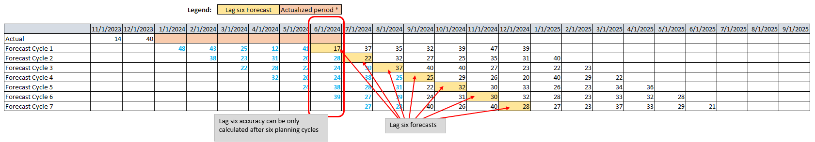
Lags
Lags represent the time interval between when the forecast was created and the actual forecast was realized. You can configure up to three forecast lags when you configure demand plan. For more information, see Create your first demand plan. The forecast accuracy metrics displays the analysis based on the lag intervals defined.
Forecasts for the defined lags are generated for every planning cycle and the accuracy metrics can only be evaluated after the corresponding number of planning cycles. For example, if you choose lag six, accuracy metrics for lag six forecast will be calculated after six planning cycles.
Note
When you change the lag configuration, the drop-down values displayed are the newly selected lags. Choose Refresh Metrics to view the latest metrics. When you change the time interval (daily/weekly/monthly/yearly), or hierarchy (product/site/customer/channel) granularity, the previous lag metrics will no longer be available when you choose Refresh Metrics. The recalculation results will display the latest demand planning cycle as the only cycle in history.
Choose Export Metrics to download a detailed file that includes granular data corresponding to the aggregated metrics displayed on the web application. The downloaded file will contain the following information:
Timestamp - Forecasted Period, Forecast Creation Date, Last Actual Period, Lag
XYZ segment (smooth, intermittent, erratic or lumpy)
Granularity - Product/site/customer/channel as configured
Baseline forecasts - P10, P50 and P90
Actual demand
Metrics - Bias Units, Bias %, MAPE, SMAPE (at granular level, MAPE and WAPE are the same)
